The phase curve of a solar-system body reveals how its brightness changes as a function of its solar phase-angle, α 1. The smaller the phase angle, the greater fraction of the asteroid’s lit surface can be seen from earth (or wherever the observer happens to be) and therefore the brighter its measured absolute magnitude. At a phase angle of 0o the asteroid is fully illuminated.
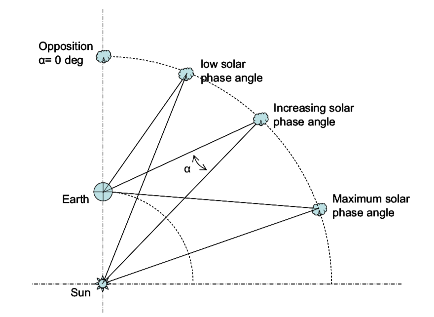
As the asteroid orbits the sun it’s not only the asteroid’s phase-angle that changes but the sun-asteroid and asteroid-earth distances are also in constant flux. This has lead to the concept of a reduced magnitude which takes account of these distances to normalise the apparent magnitudes of asteroid. This reduced magnitude is now a function of only the asteroid’s solar phase-angle and is often represented as \(H(\alpha)\) to reflect this dependence.
Plotting the reduced magnitude \(H(\alpha)\) against the phase-angle reveals the asteroids phase-curve.
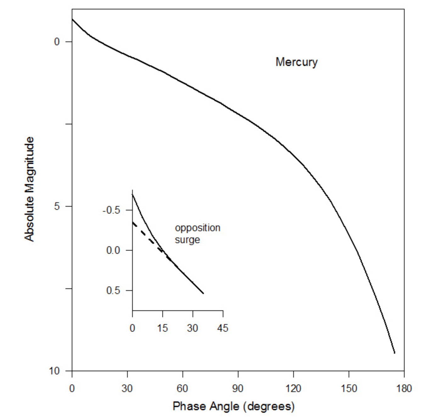
The main goal behind fitting a phase-curve to asteroid photometry is to determine a value for \(G\), the so-called slope-parameter. The \(G\) value is likely telling us something about the texture of the asteroid’s surface and its albedo (generally the higher the value of \(G\) the higher the albedo) and hints at the class the asteroid belongs to2.
A Phase-Function Model
Prior to 2012 the IAU had adopted the following 2-parameter phase function developed by Bowell et al. (1989) as a description of how an asteroid’s reduced magnitude relates to its phase-angle at any given apparition.
\(H(\alpha) = H-2.5log[(1-G)\Phi_1(\alpha)+G\Phi_2(\alpha)]\)
where:
\(H\) is the reduced magnitude at zero phase-angle. The \(\Phi\) functions detail the scattering of light in the asteroids surface and \(G\) is the slope-parameter describing the shape of the phase-curve.
\(\Phi_n(\alpha) = W\phi_{nS}+(1-W)\phi_{nL} \\ W=exp[-90.56 \times tan^2(\alpha/2)] \\ \phi_{nS}=1-\frac{C_nsin\alpha}{0.119+1.1341sin\alpha - 0.754sin^2\alpha} \\ \phi_{nL}=exp[-A_n(tan(\alpha/2))^{B_n}]\)
and
\(A_1 = 3.332 \\ B_1 = 0.631 \\ C_1 = 0.986\)
and
\(A_2 = 1.862 \\ B_2 = 1.218 \\ C_2 = 0.238\)
Note there’s often a spike in asteroid brightness known as the ‘opposition effect’ as it approaches zero phase-angle. This surge in brightness is thought to be due to a combination if physical effects including shadow hiding and other light scattering mechanisms. And a final spanner to throw into the mix is that of rotation. An asteroid’s rotation as it orbits the sun also causes its brightness to periodically fluctuate and this change is superimposed onto the phase-curve.
An Example
Let’s move onto a concrete example of fitting a phase-curve to a set of asteroid data. I’m going to use ATLAS cyan-band data taken over the past few years of the asteroid Kleopatra (MPC#216). Using ephemerides generated for each of the photometry epochs it’s trivial to convert observed to reduced magnitudes.
\(c(\alpha) = c - 5 \times log(RD)\)
where \(R\) is the sun-asteroid distance and \(D\) is the earth-asteroid distance.
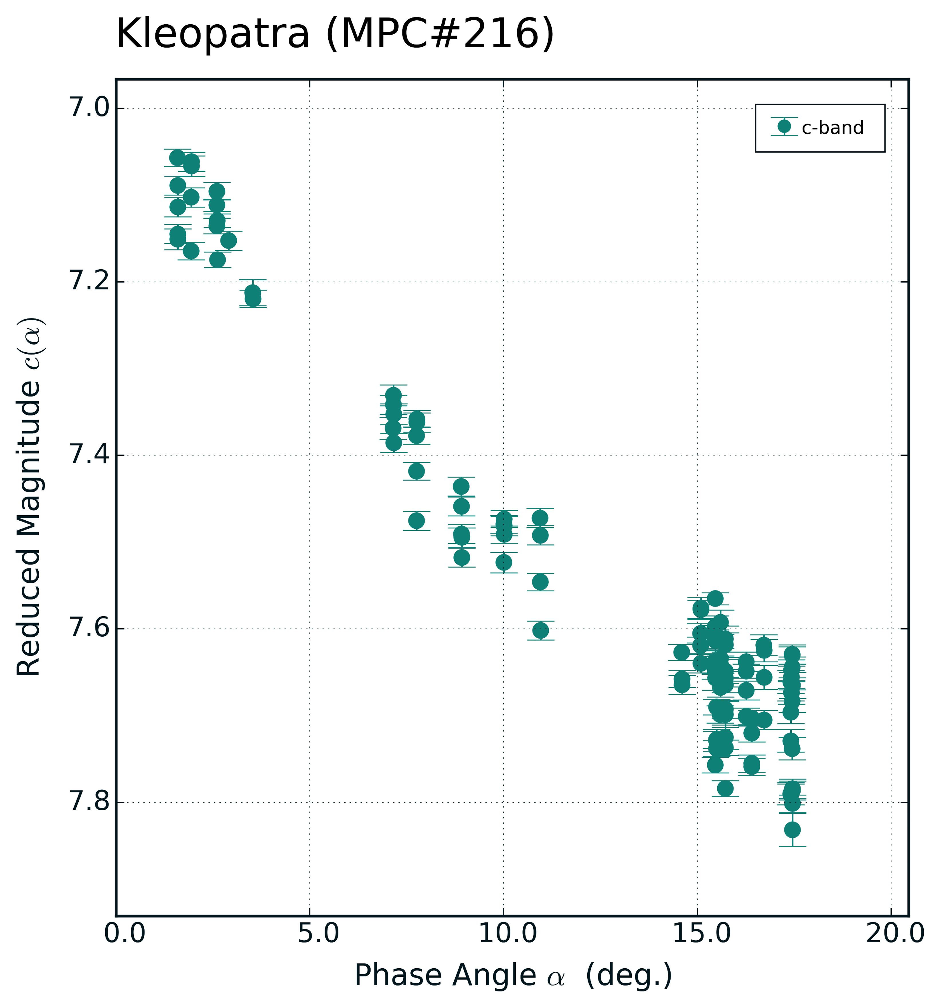
Plotting reduced magnitude vs phase-angle gives us the observed phase-curve:
Using scipy’s curve_fit, a non-linear least squared fitting routine, alongside a simplified version of the Bowell et al. (1989) model phase-function:
\(c(\alpha) = c_o-2.5log[(1-G)\Phi_1(\alpha)+G\Phi_2(\alpha)] \\ \Phi_{n}=exp[-A_n(tan(\alpha/2))^{B_n}]\)
we can fit a phase-curve to the data and output optimal values of H and G. Given the phase-function, an array of x-data (the independent variable, i.e. the phase angle) and an array of y-data (the dependent variable, i.e. our reduced magnitudes) curve_fit will iterate over various parameter values for H and G until the sum of the squares of the residuals between the fit and the input data is minimised. First an unweighted fit, where each data-point is treated equally:

Next, I reran the fitting but this time I passed the measured uncertainties of the magnitudes to curve_fit and set absolute_sigma=True to indicate that these are absolute measured errors (not just relative errors). As you can see curve_fit does well to fit a non-linear least-squares curve to the data and outputs the optimal values for H and G. Alongside the optimised parameter values curve_fit outputs a covariance matrix. The diagonals of this matrix provide individual variances of the parameter estimates therefore we can calculate the 1-std errors in the parameter values as the square-root of variance.
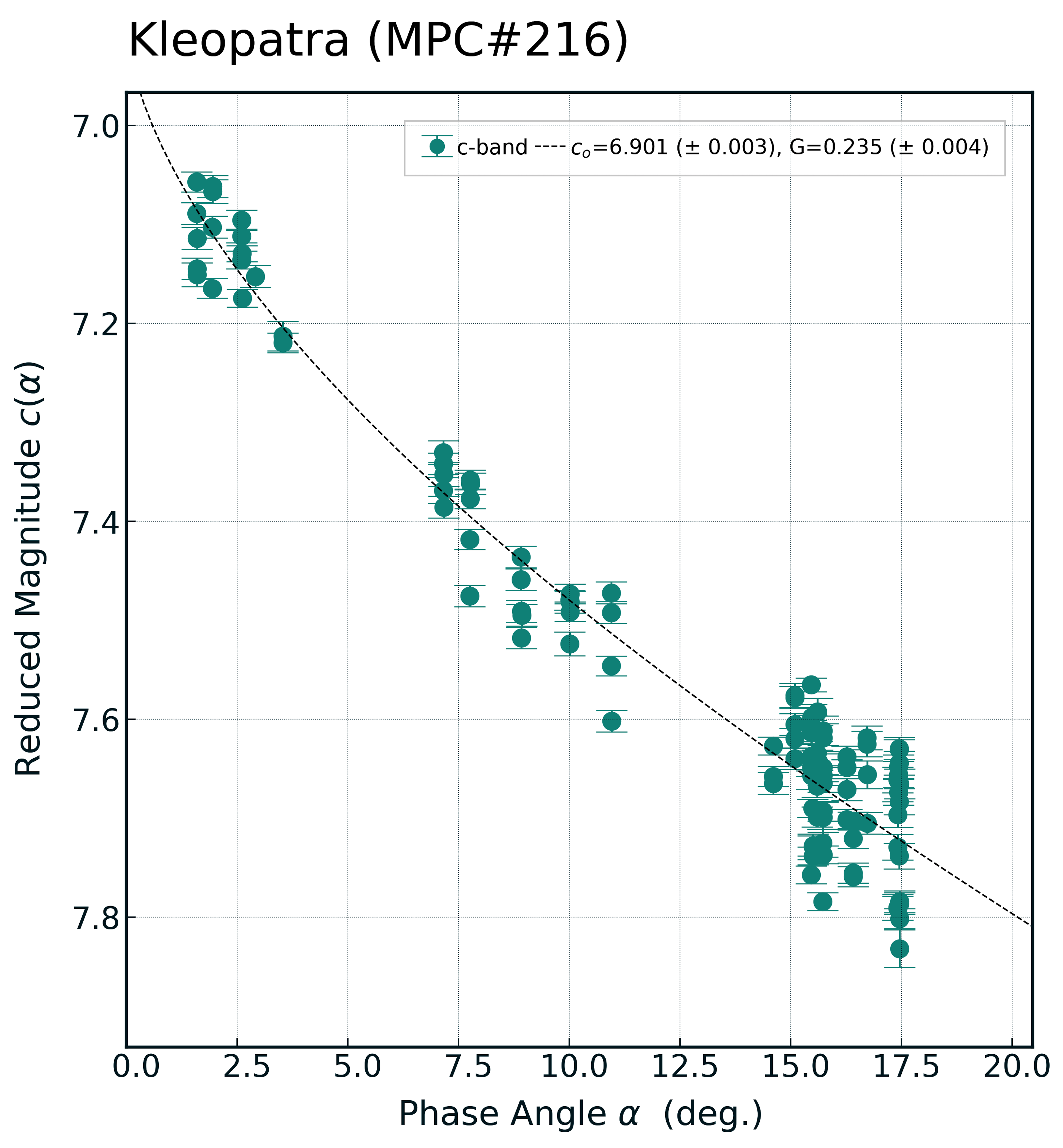
Note one huge caveat in the resulting parameter errors; we have entirely neglected the effects of asteroid rotation until now. Once we account of rotation in the error budget then these uncertainties will certainly grow.
Fitting the Full Bowell et al. (1989) phase-function
Now using the full 2-parameter version of the Bowell et al. (1989) phase-function:
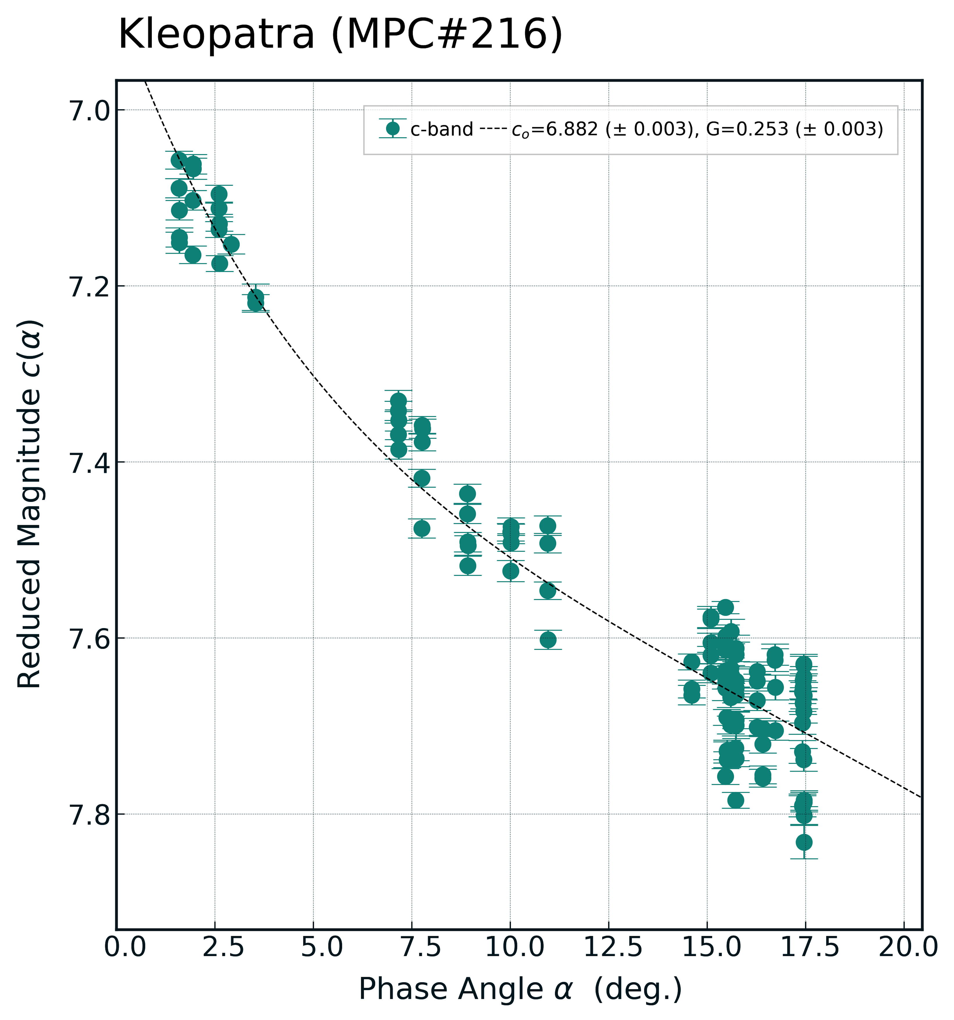
You can see more of a kink in the phase-curve causing it to arch up to a brighter c0 value than when given the simplified version of the phase-function. I’d say this accounts for the opposition effect a little better.
UPDATE May 31, 2018: The errors reported in these plot are not correct. I’ve done some better analysis of the errors reported by curve_fit. See here for more details
An Aside on Scipy’s curve_fit Routine
The curve fit routine returns:
popt : an array of the optimal values calculated for the function’s parameters that forms the moving least-squared fit to the input data.
pcov : a 2D array of the estimated covariance of parameter solutions (popt). To convert this matrix to 1-stdev parameter errors use perr = np.sqrt(np.diag(pcov)).
There are various parameters we can adjust to get a better fit but I found that (at least for my dataset) that altering the follow parameters made no difference:
| Parameter | Effect of Change |
|---|---|
p0 - inital estimate of H and G |
No change to final values or errors |
bounds – bounds for H and G values |
No change to final values or errors |
method – least squares optimisation method |
No discernable change to final values or errors |